Are All Fast Radio Bursts the Same?

Author: Lucca S. de Mello^†
Mentor: Charles L. Steinhardt^‡
Editor: Laura Lewis

^†ldemello@caltech.edu, Caltech
^‡steinhardt@nbi.ku.dk, Cosmic Dawn Center

Abstract: In 2007, astronomers discovered highly energetic, millisecond-long radio waves of extragalactic origin. These Fast Radio Bursts (FRBs) are poorly understood, and there is no definitive explanation for their origin yet. Using a novel machine learning technique, we have made significant progress toward determining whether FRBs can be separated into discrete subclasses, or if all FRBs are instances of the same astrophysical phenomenon. The technique consists of modeling the entire intensity-versus-time curve of these bursts as vectors in a high-dimensional space and clustering these vectors in two dimensions. We expect that grouping FRBs by their physical properties will also group them by their physical origin.

Background

With advances in telescope technology, humanity has recently acquired the ability to observe the sky more
closely, noticing fascinating changes that occur within the span of a millisecond. In 2007, a new class of astronomical object was discovered: fast radio bursts, or FRBs (Fig. 1). FRBs are highly energetic¹ pulses in the radio spectrum that last for approximately two milliseconds at most. Due to their very recent discovery, little is known about them. Thus, the purpose of this project is to explore this field by further investigating the origin and properties of FRBs.

The high energy and short duration of FRBs make them an especially intriguing class of astronomical object. The special theory of relativity asserts that causality travels at the speed of light. So, in the span of a millisecond, causality travels approximately 300 km. This implies that the diameter of the source of any signal with a duration of one or two milliseconds – the typical duration of an FRB – is on the order of 300 km or smaller, otherwise a complex (and thus unlikely) synchronization mechanism would be required for the bursts to be so short. Relative to distances on an astronomical scale, the order of hundreds of kilometers is fairly small.

It is also known that this mysterious source, although small, must be associated with some extremely energetic astrophysical process¹. We know this because, in spite of their short duration and the cosmological distances they travel before reaching us, FRBs are as bright in the radio frequencies as a galaxy when viewed from Earth [1].

FRB science is a nascent but thriving field of astronomy. Although the dataset is still limited, the host of instruments scattered throughout the world listening for new FRBs will give us an accelerating influx of data, which can help us further understand the nature of FRBs. We have already observed that they originate from the entire sky, not just from directions coplanar with the Milky Way³, implying that most of them are of extragalactic origin⁴. Additionally, likely candidates for what could be the source of FRBs have been identified; these include neutron stars [2] and black holes. However, due to the very recent discovery of FRBs, there is currently no definitive explanation for what astronomical object is the source of FRBs, and we are currently far away from truly understanding what they are.

FRBs are not the only kind of short-duration, high-energy burst of radiation that has been observed. There are also the gamma-ray bursts (GRBs), which are longer and brighter than FRBs. GRBs have been studied for far longer – since the late 1960s – so they are better understood. Indeed, one important milestone in GRB study has been their separation into two discrete classes, “short” and “long”⁵. The realization that not all GRBs are the same was important because, by studying these classes separately, we were able to connect each of them with an astrophysical origin: we now know that “long” GRBs are generated from the collapse of massive stars, while “short” GRBs come from neutron stars⁶. This naturally raises the question of whether or not the situation for FRBs is similar to that of GRBs. Are all fast radio bursts the same?

Goals

Despite the important advancements that have been made in the process of understanding FRBs, the key step of classification has not yet been realized. As a result, it has not been possible to connect FRBs to an astrophysical origin – or origins. So the problem we chose to tackle in this research project was that of classifying FRBs.

To this end, we have applied a novel machine-learning technique known as “dimensionality reduction,” which has recently proven successful in solving the long-standing classification problem for gamma-ray bursts (GRBs)⁷. It was known that gamma-ray bursts appear to have two types – called “short” and “long”, as previously discussed – but it had not been possible to unambiguously separate these two types of objects. For example, some “short” GRBs are actually longer in duration than some “long” GRBs.

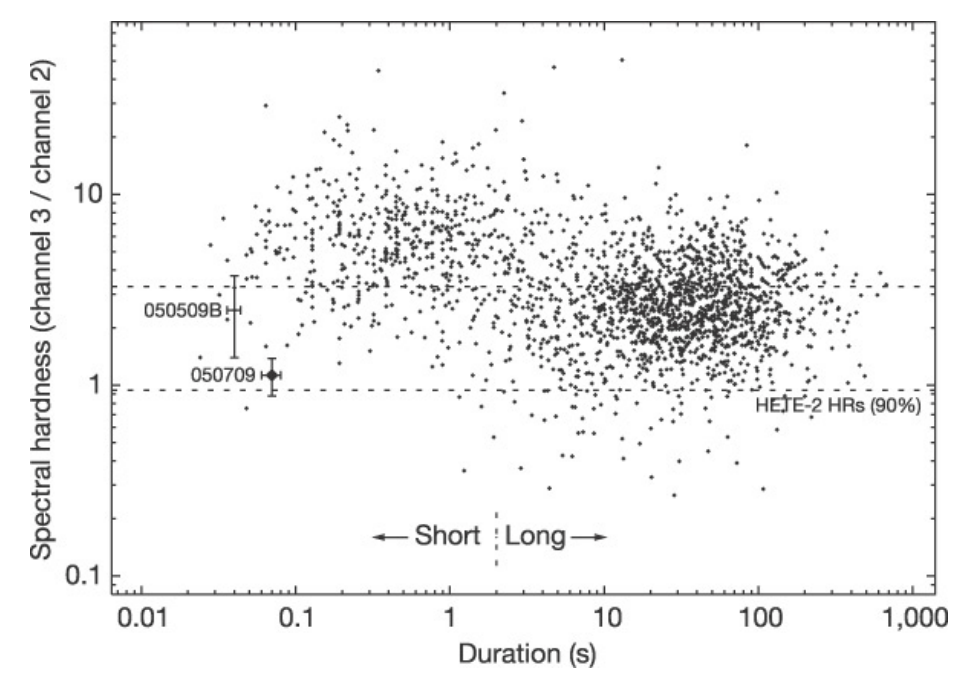
Earlier attempts at classifying GRBs took the light curve – the curve of intensity [3] versus time, integrated over all frequency channels – and make a small number of summary statistics (such as the duration of the GRBs) which lend themselves easily to physical interpretation. However, this always resulted in some ambiguous objects, which might have been either short or long, as Fig. 2 exemplifies.

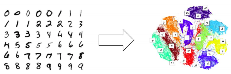
To solve this problem, instead of only using two measurements, all of the data were use. The challenge with this is what is known as “the curse of dimensionality”⁹. Suppose we want to plot objects in N dimensions, where N is the number of measurements. As N increases, so does the sparsity of the data points, meaning that all objects appear to be dissimilar in many ways. The solution was to use what is known as a dimensionality-reduction algorithm. As the name suggests, dimensionality-reduction algorithms take in a set of high-dimensional vectors that model some dataset, then cluster those vectors in a lower-dimensional space – usually in two dimensions – grouping them in a way that preserves the structure of the high-dimensional data. This means that, in the low-dimensional output space, similar objects stay close in and dissimilar objects stay distant. This idea is illustrated in Fig. 3.

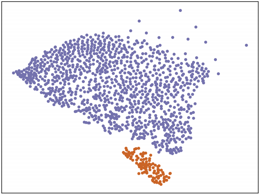
The result was Fig. 4, which shows two discrete categories of GRBs, with every object unambiguously classified as either short (orange) or long (purple). Since the problem of classifying GRBs appears to be similar to the problem of classifying FRBs, the specific goal of this project was to make progress on the latter by applying a promising technique that worked on the former. That is, our ultimate goal was to get something similar to Fig. 4, but with FRBs instead of GRBs [4]. Failure in doing so would indicate that either:

1. FRBs are, in essence, all instances of the same astrophysical phenomenon.
2. FRB subclasses do exist but may not be easily revealed by dimensionality reduction alone.
3. Unlike GRBs, FRBs can only be classified in a continuous spectrum.

Methods

As previously discussed, clustering the FRBs by representing each burst as a collection of summary statistics has not been a successful approach. So, instead, our technique consists of clustering the FRBs by the “similarity” of their light curves. For example, some FRBs have light curves that end just as abruptly as they start, while others have an exponential fallout tail after their maximum, like the burst “rings” for a period of time after peaking. Another component of this intuitive notion of similarity is that we are only concerned with the shape of the light curve; that is, if a light curve is simply a scaled-up version of another, we consider them to be similar. This is because the scaled-up (but otherwise similarly-shaped) light curve is simply a more intense version of the latter curve. Intensity should not be a factor because FRBs that appear to be more intense may simply be closer to us, so letting the bursts’ intensity affect their classification could lead to the FRBs being grouped by their sources’ proximity to Earth. Proximity is neither an intrinsic property of the FRB nor of its source, so such a clustering would be physically meaningless. For more details on the similarity of FRB light curves, see Fig. 5.

Quantitatively, we can encode the similarity of these light curves by processing the light curves into vectors in a way that:

1. Uses the raw light-curve data instead of summary statistics, making no assumptions on how strongly each physical measurement of the FRBs should influence the classification. Consequently, the clustering process is dictated by the raw data and nothing else.
2. Encodes the entire light curve. In practice, this means that it must be possible to reconstruct the light curve of an FRB from the vector representing it. In other words, the process of transforming FRBs into vectors must be reversible. As a result, our approach has perfect information on the light curves being clustered.
3. Ensures that the distance between two vectors is indeed a measure of dissimilarity in topology, or shape, of the corresponding light curves.

Since each vector stores all the information we need to reconstruct the corresponding light curve, the vectors are in a very high-dimensional space. Vectors are something we can naturally cluster, so it would stand to reason that the next step is to simply apply any clustering algorithm to the result. However, as discussed in the previous section (Goals), this would not give satisfactory results because of the “curse of dimensionality,” so we must apply a dimensionality-reduction algorithm.

The dimensionality-reduction algorithm we chose is the t-distributed stochastic neighbor embedding, or t-SNE. t-SNE assigns each high-dimensional data point to a temporary position in the low-dimensional space, called a “map point” [5], and gradually updates these positions in a way that attracts similar objects to each other and repels the objects that are dissimilar.

One physical analogy for how this is accomplished is as follows. First, the map points are connected to each other by springs. The smaller the distance between two high-dimensional data points, the stiffer the spring connecting their map points. As a result, map points are attracted if they are far apart but their corresponding objects are close. If two map points are close while their corresponding objects are dissimilar, they are repelled. Then, this system evolves until it reaches equilibrium. The equilibrium state associates each data point to its position in the low-dimensional space. For an illustration of what would result from this, refer again to Fig. 3 as the dimensionality-reduction algorithm used to compute that example was, in fact, t-SNE.

The example of classifying hand-drawn digits also illustrates how t-SNE preserves the macroscopic structure of the objects being clustered: fours look like nines, so those two clusters end up together; nines look like sevens, who
look like ones, etc. This structure-preserving property is essential for our goal of clustering FRB light curves by topological similarity, which is why we chose t-SNE for this project. Additionally, the previously-discussed success in unambiguously clustering GRBs (Fig. 4) was also accomplished using t-SNE, further motivating our choice of dimensionality-reduction algorithm.

Results

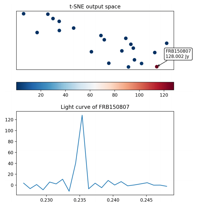
After fitting t-SNE to the processed, high-dimensional data and calibrating the algorithm’s parameters, we have obtained Fig. 6 as our program’s final output. As our figure illustrates, we have separated twenty-one FRBs into two groups: one group containing seven FRBs and the other containing fourteen. Recall that our goal was to obtain something similar to Fig. 4, but with FRBs instead of GRBs. In Fig. 4, the physical interpretation of the two subclasses is known: the orange cluster represents “short” GRBs, and the purple cluster represents “long” GRBs. Indeed, the short/long separation of GRBs was known before t-SNE was applied to GRBs (Fig. 2). Unlike GRBs, however, FRBs are still too shrouded in mystery for us to make a probable physical interpretation of the clusters in our result.

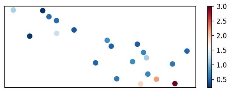
There is a significant variation in the measured intensity of FRBs. As previously discussed, while an FRB’s higher measured intensity may be an intrinsic property of the burst, it may also result from that FRB having originated closer to Earth. So, to ensure that our program is not biased by FRB intensity – that is, to show that we are not clustering FRBs by their proximity to Earth – we have also produced Fig. 7-8, in which FRBs are colored by peak intensity.

If our algorithm were biased by intensity, the resulting plot would have been, at least approximately, a spectrum from the “low-intensity” colors to the “high-intensity” colors. Instead, these figures show a mostly diverse distribution of FRBs, with both clusters containing bursts in the mid- and low- intensity ranges. The very few bursts that are in the high-intensity range are in the same cluster, but the previous observation – coupled with the fact that the light curves were normalized by peak intensity – leads us to believe that this is most likely not indicative of bias. Of course, a larger sample size is necessary for any definitive assertions on bias, or lack thereof, to be made.

Our program and the clustering we have obtained from it are both preliminary, but they are the first of their kind. Crucially, the quality of the classifications it produces will only increase with the amount of data it is given. With the global community of radio astronomers currently listening for FRBs, the amount of available FRB data is certain to grow in an accelerating fashion. We believe that, if our program is adapted to make full use of this progressively larger volume of data, it will be a significantly useful tool in solving the puzzle of FRBs.

Conclusion

We have developed a program that, given a standardized set of raw FRB data, clusters the FRBs by the similarity of their light-curves. Our program is dictated by the raw data alone, making no assumptions on how strongly each physical measurement of the FRBs should influence the classification. It has perfect information on each light curve being clustered, and everything indicates that it is not biased by each source’s proximity to Earth. Our program employs t-SNE, an algorithm that was successful in a problem very similar to that of classifying FRBs. The motivation for doing so is that we expect that grouping FRBs by their physical properties will also group them by their physical origin.

Our preliminary results imply that our program for processing and grouping FRB light-curves is a promising candidate as a solution to the challenge of classifying FRBs. Further, it implies that more definitive classification results obtained by running our program on a larger dataset will likely be unbiased with respect to proximity.

While our result does represent a necessary first step in the challenge of classifying FRBs, the problem has not
been solved. Due to several technical factors related to the very recent discovery of FRBs, we only had access to
a small sample size. One of the most difficult parts of studying FRBs is that the raw data is not easily accessible, as
there is no publicly-available catalog of raw FRB data yet [6]. Additionally, raw FRB data is stored in a large variety of file formats; if there were a standard for storage of raw FRB data, classification studies would probably advance much faster. For these two reasons, conclusive further research in this area will likely required the creation of a catalog of raw FRB data that uses a standardized file format [7].

Moreover, the algorithm developed in this project can only produce meaningful results if the dataset uses the same sampling period across all FRB recordings. This means that most datasets are not compatible with each other; some datasets, such as the one used in this project, are not even consistent within themselves. And, as previously discussed, FRB data is still limited. So, to obtain more definitive classification results through our algorithm, further research may have to wait until there is a larger collection of FRB observations with practically identical time resolutions.

Are all fast radio bursts the same? We do not know, and it may still take time until it is possible to answer this
question. But we have developed a tool that can be very useful in doing so; all we need is more data. We hope that,
with a large, standardized, and easily accessible catalog of raw FRB data, the use of machine learning in the classification of FRBs will prove to be a powerful way in which the nature of these mysterious objects can be better understood.

Acknowledgements

This research project is a part of, and was made possible by, the SURF program. I thank the Caltech Student-Faculty Office for their support, and I thank my mentor, Charles L. Steinhardt, for his help in executing this project. I think Duncan Lorimer for helping us obtain raw FRB data.

Appendix

The data and code used in this research can be found in this Github repository.

For this project, twenty-seven plaintext files of raw FRB light-curve data were acquired with the help of Dr. Duncan Lorimer. So that the light curves may be meaningfully compared, the twenty-one files (of those twenty-seven) whose data used the mode sampling period (0.97 ms) were selected. These 21 FRBs are in the “data” directory of the linked repository. The other six are in the “bad data” directory, which is not used by the program. The table below shows which 27 FRBs were used in this project, ordered by when they occurred [8]. The first 21 FRBs in the table were recorded with practically the same sampling period, and therefore can be meaningfully compared using our program. Accordingly, these twenty-one FRBs are the ones in Fig. 6-8.

FRB	Sampling Period
FRB010125	9.70000E-04
FRB010621	9.70000E-04
FRB090625	9.70000E-04
FRB110214	9.76562E-04
FRB110220	9.76562E-04
FRB110626	9.76562E-04
FRB110703	9.76562E-04
FRB120127	9.76562E-04
FRB121002	9.76562E-04
FRB130626	9.76562E-04
FRB130628	9.76562E-04
FRB130729	9.76562E-04
FRB131104	9.76562E-04
FRB140514	9.76562E-04
FRB150215	9.76562E-04
FRB150418	9.76562E-04
FRB150610	9.76562E-04
FRB150807	9.76562E-04
FRB151206	9.76562E-04
FRB151230	9.76562E-04
FRB160102	9.76562E-04
FRB171209	7.81221E-05
FRB180301	1.17000E-03
FRB180309	1.25016E-04
FRB180311	1.51286E-03
FRB180714	1.39082E-03
FRB180923	4.88281E-03

References

1. L. Billings. A Brilliant Flash, Then Nothing: New Fast Radio Bursts Mystify Astronomers (2013).
2. D. Lorimer. A bright millisecond radio burst of extragalactic origin (2007).
3. M. Caleb et al. The first interferometric detections of Fast Radio Bursts (2017).
4. M. Kiyoshi et al. Dense magnetized plasma associated with a fast radio burst (2015).
5. C. Kouveliotou et al. Identification of Two Classes of Gamma-Ray Bursts (1993).
6. E. Nakar. Short-Hard Gamma-Ray Bursts (2007).
7. C. Jespersen et al. An Unambiguous Separation of Gamma-Ray Bursts into Two Classes from Prompt Emission Alone (2020).
8. R. M. Shannon et al. The dispersion-brightness relation for fast radio bursts from a wide-field survey (2018).
9. R. E. Bellman. Adaptive control processes: a guided tour (1961).
10. D. Michilli et al. An extreme magneto-ionic environment associated with the fast radio burst source FRB 121102 (2018).
11. C. D. Bochenek et al. STARE2: Detecting Fast Radio Bursts in the Milky Way (2020).
12. J. P. U. Fynbo et al. The optical afterglow of the short gamma-ray burst GRB 050709 (2005).
13. A. Shahmoradi. Hardness as a spectral peak estimator for gamma-ray bursts (2010).
14. Pedregosa et al. Scikit-learn: Machine Learning in Python (2011).

Footnotes

[1] Fig. 5 of On the Normalised FRB Luminosity Function shows the luminosity function of FRBs, i.e. the number of FRBs per luminosity interval. Comparing it to the luminosity function of galaxies shows that, in general, the luminosity of FRBs is indeed similar to that of galaxies.

[2] Some FRBs are polarized, which indicates that at least those FRBs were emitted from a specific kind of neutron star called a magnetar¹⁰. Indeed, the first FRB to have been linked to a known source, FRB200428, was found to originate from a magnetar¹¹.

[3] By “intensity,” we mean Spectral flux density, measured in Janskys (Jy).

[4] Though we did not assume that the number of FRB subclasses, if they exist, is only two.

[5] Map points are computed using probabilistic methods beyond the scope of this paper.

[6] There is frbcat.org, a publicly-available catalog of FRB data, but it does not store raw FRB data; it is limited to summary statistics. While these are useful in general, using summary statistics has not been a fruitful strategy in the challenge of classifying FRBs.

[7] Or, alternatively, the extension of frbcat.org into one such catalog.

[8] Not necessarily when they were discovered; many FRBs, including the first one ever found, are discovered from old archival data.