Convolutional Neural Networks as Efficient Emulators for Atmospheric Models

Author: Berlin Chen
Mentors: Hai Nguyen, Derek Posselt
Editor: Michael Yao

Abstract

We used Convolutional Neural Networks (CNNs) to emulate the physics of the atmosphere in order to bypass solving partial-differential equations (PDEs) explicitly, which cuts down on computational cost. This is important because in the past, the models used to produce reliable weather forecasts required a computationally complex calibration.
We let the CNNs learn on a 4-dimensional (longitude x latitude x height x time) geophysical dataset, with a separate CNN for each height index. After a series of experiments we conducted following implementation, we found that zero-padding the data, varying time scale, and changing sample space had little effect on the CNNs’ performance, and that there was little correlation between training data size and error. We also observed that given the same training-data size, the CNNs with a more complex configuration (more sets of weights) actually performed worse.

1 Background

1.1 Variability Quantification

Reliability of weather forecasts has a variety of important consequences. Certainly, reliable weather forecasts bring people convenience of knowing when to bring an umbrella or when to stay at home rather than go to the supermarket. Our economy also has a stake in reliable weather forecasts, as natural disasters incur billions of dollars in damage each year [1]. $^1$

Improving the reliability of weather forecasts, however, can be a challenge. In particular, initial conditions of the forecast model (such as referential sea-level pressure) can differ from reality. Because the underlying mechanisms governing the atmospheric behavior can be unstable, small changes in initial conditions can lead to wildly different predictions.

One way to characterize variability is to treat the value of each parameter not as a unique value, but rather as a probability distribution of values. In this context, prediction is the calibration of the probabilities of a parameter having certain values in the future, given the current measurement of some parameters. Bayes’ theorem allows us to quantify this information:

$P(A | B) \; \propto \; P(A) \cdot P(B | A)$

where $P(A|B)$ denotes the probability of $A$ having certain value given that $B$ has certain value. In our model we let $B$ be the parameter we would like to predict and $A$ be the parameter corresponding to a control variable.

Repeated simulations evaluating the sensitivity of $B$ in response to changes in $A$ can be done by computing the solutions to algorithms approximating partial-differential equations (PDEs) governing the underlying physics; however, this method comes with high computational cost $^2$ . As a potential solution, we speculated that, by using techniques in machine learning, we will be able to scale down the computer runtime without compromising the accuracy significantly.

1.2 Machine Learning and Neural Networks

Machine learning essentially describes the process of approximating input-output relationships. Toddlers learn by observing and drawing connections (as opposed to memorizing formal rules). In the same way, we can analogously design a procedure that directs computers how to acquire information about a function, instead of coming up with hard-and-fast rules for arriving at a solution. In practice, this means that, instead of computing desired outputs from given inputs, one would feed into the computer many input-output pairs and let the computer learn the mapping. This technique is highly relevant when the function is too complex to solve analytically $^3$ .

The machine-learning technique that we used to realize this concept is called a $\textit{neural network}$ . For the most part, a neural network can be represented as a computational graph. One can think of a computational graph as an assembly line consisting of a collection of workers, each doing a separate task. $^4$ . Moreover, there is an established workflow among the workers, such that a worker may work on something that is produced by another worker. In our case, instead of manufacturing material goods, each worker in a computational graph does a simple task such as addition of two numbers. Although each worker contributes only a simple task, cooperation among the workers can result in complex calculations, which is why neural networks are so expressive. $^5$ . Figure 1 gives an example of a computation graph.

Figure 1: An example of a computational graph [4]. One can think of each bubble as a worker doing a simple task such as addition of two numbers (or, in the case of the bottom two bubbles, delivering a number). The arrows specify the workflow among these workers.

In neural networks, the nodes in the graph (the workers) are organized into non-mutually exclusive subsets, called $\textit{layers}$ . Figure 2 illustrates an example layer. The nodes in a layer, in turn, can be organized into $\textit{inputs}$ , $\textit{weights}$ , and $\textit{outputs}$ , with inputs being the parents of weights and weights being the parents of outputs (the node is a $\textit{parent}$ of another node when the latter’s calculation depends on the former’s output). Whereas weights are constants, variable outputs are defined by taking dot products of parent weights with inputs, and then transforming the result with some function (called the $\textit{activation function}$ ) so that an output of one layer can be used as an input to another layer.

Figure 2: An example layer of a neural network (taken from [5] with modification). To better visualize such a layer (which is a computational graph), it is flipped sideways, and the bubbles are redrawn into boxes and circles to distinguish between input and output layers (weights are omitted).

Every neural net has an $\textit{input layer}$ and an $\textit{output layer}$ . The input layer contains all the nodes with no incoming edges, while the output layer contains all the nodes with no outgoing edges. A layer that is neither input layer nor output layer can be called a $\textit{hidden layer}$ . In this context, a run of the neural nets means feeding data into the input layer and observing values of the output layer’s outputs.

To implement a typical neural network model, we must first train the model on many input-target pairs by running the neural network with some or all of the inputs. We may determine the neural network’s performance by using some error measures (such as the mean squared error, or MSE, of the neural network’s outputs with respect to corresponding targets). To the minimize error measures, we may update the neural network’s weights. $^6$

Generally, a model is only as good as the training data, and so the neural-network approach is domain specific and cannot be easily generalized from, say, one geographical region to another [4]. The model, however, is advantageous in speed. Using machine-learning techniques, we bypass the task of solving PDEs (partial differential equations), which is traditionally where the bulk of computation takes place. Consequently, the runtime of neural-net predictions will be orders of magnitude less than those of PDE solvers. Hence, if our speculation is sound, then neural nets could address the need for speeding up repeated simulations of differing initial values, which, as mentioned earlier, is a crucial contributor to the characterization of weather-forecast uncertainty.

1.3 Convolutional Neural Nets (CNN)

The distinctive feature of a CNN, which is the type of neural networks we used for this project, is the inclusion of one or more convolutional layer(s). To understand how the output of a convolutional layer is related to its inputs, one can imagine applying ( $\textit{i.e.}$ taking the dot product and applying some activation function of) a matrix of weights (with dimensions less than or equal to the input’s) repeatedly across the input space.
It has been shown that a CNN can achieve remarkable accuracy when it is applied to the task of labeling certain features in some spatially-meaningful data (such as images and videos) [9]. Therefore, since the atmospheric behavior for the kinds of data we use is also spatially meaningful, a CNN is a promising candidate.

1.4 Nature Run Dataset

For our experiments, we used the Nature Run dataset. It is generated by the model in 5-minute intervals from 00 UTC 22 Nov 2006 to 06 UTC 23 Nov 2006 (a total of 30 hours) $^7$ , and is comprised of 4-D grids of size 2701 x 1999 x 74 x 360 (longitude x latitude x height x time), which corresponds to observations that are 1.3 km apart, 74 levels tall $^8$ , and span 30 hours. Each grid contains information about a certain geophysical measurement, such as water vapor. For our experiment, we took grids containing information about water vapor, air temperature, and winds. We merged those data in the third ( $z$ ) dimension, which would have $74\cdot 4 = 296$ indices. For the sake of computational feasibility (and also to reduce correlation between data points), we took every ten steps in the first two dimensions. Consequently, the dataset we used is of size 270 x 200 x 296 x 360.

2 Experiments

2.1 Preliminary Results

Prior to designing and running the experiments, we trained the CNNs on the time interval from the $0^{th}$ to the $1^{st}$ hour of Nature Run and visualized its prediction on the 2nd time step (5 minutes from the beginning of Nature Run) with the input being the 1st time step (the beginning of Nature Run). Figure 3 illustrates the heat maps produced by our CNN that was trained to predict data with $z$ index equals 11, which corresponds to a vertical layer of water-vapor data. The values of both the prediction and the data we hope to predict (which we will refer to as “truth” or “target”) are standardized.

Figure 3: Prediction of a single time step with input being some training data. This shows the heatmaps produced at the $11^{th}$ vertical ( $z$ ) index. The heatmap to the left is CNN’s prediction, and the heatmap to the right is the target. The heatmap in the middle is their difference. All values are standardized.

Figure 3: Prediction of a single time step with input being some training data. This shows the heatmaps produced at the $11^{th}$ vertical ( $z$ ) index. The heatmap to the left is CNN’s prediction, and the heatmap to the right is the target. The heatmap in the middle is their difference. All values are standardized.

To measure loss, we divided the variance of the residual ( $Y-\hat{Y}$ ) by the variance of the ground truth (we will call this measure $\textit{loss}$ ). This measure allowed us to both quantify how well the model fits and detect instances when the algorithm is merely guessing randomly (in which case we obtain 1 using this measure). The data illustrated in Figure 3 has a loss values of $0.0078$ . We judged that a low loss value and visual similarity in heatmaps mean the CNNs performed quite well in minimizing the training error. However, note that it conveyed little information about the generalizability of the CNNs.

Additionally, we trained the CNNs on the interval from the 6th to the 30th hour of Nature Run and let it predict the same 24-hour interval it was trained on (and so the input corresponding to the zeroth time step is the ground truth while all subsequent inputs are predictions made by the CNNs), in order to gauge how well the CNNs may generalize inputs generated by themselves. Figure 5 illustrates snapshots taken at various time steps, along with the plot of the loss as a function of time steps predicted $^9$ . We observed that the CNN started with fairly accurate predictions (which is somewhat expected since little generalization is needed to accurately predict the first few time steps); however, after around the $24^{th}$ prediction, the quality of prediction diminished, as evident from the blurred resolution of the heatmaps.

2.2 Variable Testing

Having these preliminary results, we ran a series of five experiments in an effort to understand how various parameters affect the behavior of the CNN.

First, we tested whether using zero padding significantly affects CNN’s prediction accuracy. $\textit{Zero padding}$ is a technique that keeps the input dimension consistent by expanding the dimension of some input data and filling in the empty entries with zeros.) Zero padding is relevant in our pipeline because for each prediction, there exist data points at the “edges”, where we could not obtain enough information necessary to make a prediction. Consequently, we need zero padding to address such loss, but we would like to access its effect on CNN’s prediction accuracy.

To establish basis for comparison, we introduced another padding scheme: instead of filling in zeros, we filled in the ground truth ( $\textit{true padding}$ ). Using the same (default) CNN configuration and same training/prediction dataset, we could compare the prediction using the two padding schemes. Based on the results (see Figure 6) we observed that there is very little difference in CNNs’ performance between zero padding and true padding. $^{10}$

Secondly, we tested whether training the CNNs to output the spatial data that is two or more time steps away from the input data (the default is one time step) would yield better results ( $\textit{i.e.}$ whether larger time increment would lead to higher prediction accuracy). It is possible that predictions done on a coarser time scale yield better results. The reason is that finer meshes could cause CNNs to primarily pick up noise in the data, instead of the desired physical interactions.

To examine this possibility, we trained two versions of CNNs, $\textit{ceteris paribus}$ : in the first version, the CNNs would be trained to predict data 1 time step away from the input, whereas in the second version, the CNNs would be trained to predict 2 time steps away from the input. From our result (see Figure 7), we did not observe any noticeable improvement in prediction accuracy for CNNs trained with larger time increment. $^{11}$

Thirdly, we tested how well the model learned by our CNNs extrapolates to time intervals outside of the training data’s time interval (ideally, the model learned by the CNNs would generalize to any given time interval). To that end, we compared predictions where the first input is taken from the training data, to predictions where the first input lies outside the training time-step interval. In this case, comparison entails using the same CNN models to predict different ranges of time steps, one inside and one outside the training time-step interval, and observing the discrepancy in accuracy. Based on the result (see Figure 8), we observed very little difference in CNNs’ performance. In this case, even as predictions were made on different time intervals, the quality of prediction does not differ significantly. This supports that the time interval for predictions has little influence on the quality of predictions.

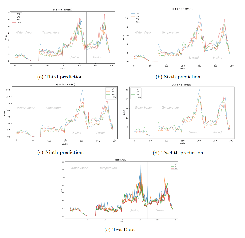
Fourth, we assessed the performance of the CNNs as a function of the available sample size. This is motivated by the observation that training the CNNs with all available training data until convergence is demonstrably infeasible given our time budget and computing resources. To that end, we trained the CNNs given 1, 2, 5, and 10 percent of all available training data (all configurations have a training time-step interval of six hours).

Based on our result (see Figure 9), we observed a lack of correlation between prediction accuracy and training data size. Although this does not inform us about the performance of CNNs with training data larger than 10 percent of total available data, the lack of correlation between prediction accuracy and training data size at least provides a reason to believe that the CNNs trained with 2 percent of total available data do not perform consistently worse than those trained with 10 percent.

Finally, we assessed how the CNN’s prediction accuracy would be affected if we make the CNN’s architecture more complex $^{12}$ , in hope that, given the complexity of the task, a more complex architecture can develop a more accurate model that yield better performance.

From Figure 10, it seems clear that CNNs with higher complexity have lower prediction accuracy. A possible explanation is that, in the case of more complex CNNs, there are more parameters in the CNNs to tune, and so the space of all possible models (the $\textit{hypothesis space}$ ) is larger. This implies that the CNNs in this case would be more prone to overfitting, explaining the lower prediction accuracy.

Figure 4 provides a visual summary of all experiments mentioned.

Figure 4: Visual summary of the five experiments aimed to better understand how various parameters affect the CNNs’ prediction accuracy. We found that adding zero padding, adjusting time increments, varying time interval for prediction, and varying training sample size all had little noticeable affect on prediction accuracy. A more complex CNN, in fact, resulted in decrease in prediction accuracy.

Figure 5. Visualization of repeated prediction over a 24-hour interval. $t$ in this case refers to the temporal index. For each temporal index, the upper left panel is the CNN’s prediction, the upper left is the target, the lower left is the difference between prediction and truth, and the lower right is the loss as a function of temporal indices. (Note that the y-axis is inverted.)

Figure 6: RMSE plots showing the predictions by CNNs with zero padding and by CNNs with true padding (Experiment 1). Each value of the X-axis (level) refers to a CNN trained to predict the Nature Run dataset given a vertical index. Y-axis refers to the CNN’s non-standardized RMSE (to show the physical aspect of data). Vertical lines are added to distinguish one type of data from another. This interpretation of X- and Y-axes applies to Figures 7, 8, 9, and 10 as well.

Figure 7: RMSE plots showing the predictions by CNNs trained to predict data 1 time index away from the input and the predictions by CNNs trained to predict data 2 time indices away from the input (Experiment 2). In addition to comparing the predictions across the same data, we compared predictions across the same number of predictions made. Figure 7e shows the result of both congurations making a single prediction (we also gathered the CNN’s RMSE on the test data).

Figure 8: RMSE plots showing the CNNs predicting two time intervals, one overlapping with the
training time interval and the other lying outside of it (Experiment 3).

Figure 9: RMSE plots showing the prediction by CNNs trained with various available sample sizes (Experiment 4). In addition to the repeated predictions is a plot showing the predictions with
inputs being the test data.

Figure 10: RMSE plots showing the prediction by CNNs configured with different number of sliding windows (Experiment 5).

Future Works

Based on our findings, we are confident that CNNs could be refined as an emulator that efficiently quantifies uncertainties, a task crucial to reliable weather forecasts. Besides the questions we addressed in this research, there are other inquiries relevant in our assessment of our CNN implementation. For instance, we would like to know whether tuning hyperparameters, such as the learning rate for the CNNs, would lead to better performance. Also, for the CNNs to be an effective emulator for longer time intervals, we would like to further investigate principle factors that contribute to the blurring of prediction overtime. So far, we provided only qualitative assessments, and so further research is needed in order to identify the kind of quantitative assessments suitable for our purpose. Additionally, we would like to assess the CNNs’ performance beyond the Nature Run dataset.

Acknowledgements

The author would like to thank his mentors, Hai Nguyen and Derek Posselt, for their mentorship, expertise, and support. The author also would like to thank Amy Braverman, the Principle Statistician of JPL, for making this opportunity possible and for offering numerous helpful advices. The author owes much to the helpful feedback and support he received from JPL’s Uncertainty Quantification group, as well as the technical support he benefited from Bob P. Thurstans, a member of the Technical Staff at JPL’s Science Division. The author is also grateful for the abundant resources and opportunities available to him as a participant of the Caltech SURF program. Finally, the author would like to thank his family and colleagues, with whom he shares the same workspace, for their constant presence and support.

References
[1] Denning, Marty. “The Impact of Accurate Weather Forecasting Data For Business.” The Weather Company. October 27, 2015. Accessed October 20, 2017. https://business.weather.com/blog/the-impact-of-accurate-weather-forecasting-data-for-business.

[2] Rappaport, Edward N. “Loss of Life in the United States Associated with Recent Atlantic Tropical Cyclones.” $\textit{Bulletin of the American Meteorological Society}$ 81, no. 9 (March 10, 2000): 2065-073. doi:10.1175/1520-0477(2000)0812.3.co;2.

[3] Smith, Ralph C. $\textit{Uncertainty quantification: theory, implementation, and applications}$ . Philadelphia: SIAM, 2014.

[4] Olah, Christopher. “Calculus on Computational Graphs: Backpropagation.” Colah’s blog. August 31, 2015. Accessed October 21, 2017. http://colah.github.io/posts/2015-08-Backprop.

[5] Mas, Jean, and Juan Flores. “The application of artificial neural networks to the analysis of remotely sensed data.” $\textit{International Journal of Remote Sensing}$ 29 (February 2008): 617-63. Accessed October 20, 2017.

[6] Hagan, Martin T., Howard B. Demuth, Mark Hudson. Beale, and Orlando De Jesús. $\textit{Neural network design}$ . S. l.: S. n., 2016.

[7] Skamarock, William C., Joseph B. Klemp, Jimy Dudhia, David O. Gill, Dale M. Barker, Micheal G. Duda, Xiang-Yu Huang, Wei Wang, and Jordan G. Powers. “A Description of the Advanced Research WRF Version 3.” NCAR TECHNICAL NOTE, June 2008. http://www2.mmm.ucar.edu/wrf/users/docs/arw_v3.pdf

[8] Karpathy, Andrej. “Convolutional Neural Networks (CNNs / ConvNets).” CS231n Convolutional Neural Networks for Visual Recognition. Accessed October 20, 2017. http://cs231n.github.io/convolutional-networks/

Footnotes

$^1$ Of course, natural disasters are responsible for loss of lives. According to [2], freshwater flood can claim up to thousands of lives in the Americas

$^2$ Some numerical solvers have a runtime of $O(n^3)$ , with $n$ being the size of the input data.

$^3$ An example of such a relationship would be the change in rainfall as a function of a change in the value of a model parameter ( $\textit{e.g.}$ the distribution of water vapor in the geographical region).

$^4$ More precisely, a computational graph is an acyclic directed graph with each node representing a variable that is either a constant or an operation on variables represented by its parent nodes.

$^5$ The “neural networks” discussed here are limited to feedforward neural networks, the type of neural networks used in this paper.

$^6$ This can be done using some kind of backpropagation scheme, such as stochastic gradient descent.

$^7$ The ensemble of physics schemes used are Morrison 2-moment microphysics, RRTMG shortwave and longwave radiation, MYJ PBL, Monin-Obukhov surface layer, and Unified Noah land surface.

$^8$ The vertical ( $z$ ) dimension is measured in the $\sigma$ coordinate. For more information about this measure, see section 2.1 of [7].

$^9$ Note that we had not considered using zero-padding at this point, and so the heatmaps and the loss were calculated exclusive of the edges of the data.

$^{10}$ Although true padding has lower RMSE at certain $z$ indices such as $z=200$ , for the most part the RMSE of CNNs with zero padding matches closely with the RMSE of CNNs with true padding. This suggests that zero padding has little influence on the CNN performance.

$^{11}$ Although we observed CNNs trained with larger time increment (for convenience we call them “ $t+2$ ” and we call the CNNs with smaller time increment “ $t+1$ “) had consistently lower RMSEs, we also observed that the RMSE of $t+2$ is not consistently lower than $t+1$ ‘s when comparing across a single prediction, as shown in Figure 7e. Based on this, we conjectured that the driving factor that caused lower RMSE in $t+2$ is that the errors are compounded less, as it would take less iterations of $t+2$ to generate a prediction, and not that $t+2$ is a better model than $t+1$ .

$^{12}$ In particular, we increase the number of filters, such that the first convolutional layer has 64 filters and the second has 128, as opposed to 32 and 64.

Share this:

Like this:

Related

Leave a Reply Cancel reply